API
Analysis Module
This module defines analysis routines and associated machinery
Notes
Without laminate details like layup and ply properties, this module is limited to max strain analysis. However, with a third party CLPT package , the parent class Analysis can be used to extend this module to check max stress, Tsai-Wu, Tsai-Hill, etc.
-
class
bjsfm.analysis.Analysis(a_matrix: <sphinx.ext.autodoc.importer._MockObject object at 0x7f270bb7e0a0>, thickness: float, diameter: float)¶ Parent class for analysis sub-classes
Parameters: - thickness (float) – plate thickness
- diameter (float) – hole diameter
- a_matrix (array_like) – 2D 3x3 A-matrix from CLPT
-
t¶ plate thickness
Type: float
-
r¶ hole radius
Type: float
-
a¶ 2D 3x3 A-matrix from CLPT
Type: ndarray
-
a_inv¶ 2D 3x3 Inverse A-matrix from CLPT
Type: ndarray
-
static
bearing_angle(bearing: <sphinx.ext.autodoc.importer._MockObject object at 0x7f270bb7e0a0>) → tuple¶ Calculates bearing load and angle
Parameters: bearing (array_like) – 1D 1x2 array [Px, Py] Returns: p, theta – bearing load (p) and angle (theta) Return type: float
-
displacements(bearing: <sphinx.ext.autodoc.importer._MockObject object at 0x7f270bb7e0a0>, bypass: <sphinx.ext.autodoc.importer._MockObject object at 0x7f270bb7e0a0>, rc: float = 0.0, num: int = 100, w: float = 0.0) → <sphinx.ext.autodoc.importer._MockObject object at 0x7f270bb7e0a0>¶ Calculate displacements
Parameters: - bearing (array_like) – 1D 1x2 array bearing load [Px, Py] (force)
- bypass (array_like) – 1D 1x3 array bypass loads [Nx, Ny, Nxy] (force/unit-length)
- rc (float, default 0.) – characteristic distance
- num (int, default 100) – number of points to check around hole
- w (float, default 0.) – pitch or width in bearing load direction (set to 0. for infinite plate)
Returns: 2D numx2 array of plate displacements (u, v)
Return type: ndarray
-
plot_stress(bearing: <sphinx.ext.autodoc.importer._MockObject object at 0x7f270bb7e0a0>, bypass: <sphinx.ext.autodoc.importer._MockObject object at 0x7f270bb7e0a0>, w: float = 0.0, comp: str = 'x', rnum: int = 100, tnum: int = 100, axes: <sphinx.ext.autodoc.importer._MockObject object at 0x7f270bb7e040> = None, xbounds: tuple = None, ybounds: tuple = None, cmap: str = 'jet', cmin: float = None, cmax: float = None) → None¶ Plots stresses
Notes
- colormap options can be found at
- https://matplotlib.org/3.1.1/tutorials/colors/colormaps.html
Parameters: - bearing (array_like) – 1D 1x2 array bearing load [Px, Py] (force)
- bypass (array_like) – 1D 1x3 array bypass loads [Nx, Ny, Nxy] (force/unit-length)
- w (float, default 0.) – pitch or width in bearing load direction (set to 0. for infinite plate)
- comp ({'x', 'y', 'xy'}, default 'x') – stress component
- rnum (int, default 100) – number of points to plot along radius
- tnum (int, default 100) – number of points to plot along circumference
- axes (matplotlib.axes, optional) – a custom axes to plot on
- xbounds (tuple of int, optional) – (x0, x1) x-axis bounds, default 6*radius
- ybounds (tuple of int, optional) – (y0, y1) y-axis bounds, default 6*radius
- cmap (str, optional) – name of any colormap name from matplotlib.pyplot
- cmin (float, optional) – minimum value for colormap
- cmax (float, optional) – maximum value for colormap
-
polar_points(rc: float = 0.0, num: int = 100) → tuple¶ Calculates r, theta points
Parameters: - rc (float, default 0.) – distance away from hole
- num (int, default 100) – number of points
Returns: r, theta – 1D arrays, polar r, theta locations
Return type: ndarray
-
strains(bearing: <sphinx.ext.autodoc.importer._MockObject object at 0x7f270bb7e0a0>, bypass: <sphinx.ext.autodoc.importer._MockObject object at 0x7f270bb7e0a0>, rc: float = 0.0, num: int = 100, w: float = 0.0) → <sphinx.ext.autodoc.importer._MockObject object at 0x7f270bb7e0a0>¶ Calculate strains
Parameters: - bearing (array_like) – 1D 1x2 array bearing load [Px, Py] (force)
- bypass (array_like) – 1D 1x3 array bypass loads [Nx, Ny, Nxy] (force/unit-length)
- rc (float, default 0.) – characteristic distance
- num (int, default 100) – number of points to check around hole
- w (float, default 0.) – pitch or width in bearing load direction (set to 0. for infinite plate)
Returns: 2D numx3 array of plate strains
Return type: ndarray
-
stresses(bearing: <sphinx.ext.autodoc.importer._MockObject object at 0x7f270bb7e0a0>, bypass: <sphinx.ext.autodoc.importer._MockObject object at 0x7f270bb7e0a0>, rc: float = 0.0, num: int = 100, w: float = 0.0) → <sphinx.ext.autodoc.importer._MockObject object at 0x7f270bb7e0a0>¶ Calculate stresses
Parameters: - bearing (array_like) – 1D 1x2 array bearing load [Px, Py] (force)
- bypass (array_like) – 1D 1x3 array bypass loads [Nx, Ny, Nxy] (force/unit-length)
- rc (float, default 0.) – characteristic distance
- num (int, default 100) – number of points to check around hole
- w (float, default 0.) – pitch or width in bearing load direction (set to 0. for infinite plate)
Returns: 2D numx3 array of plate stresses (sx, sy, sxy)
Return type: ndarray
-
xy_points(rc: float = 0.0, num: int = 100) → tuple¶ Calculates x, y points
Parameters: - rc (float, default 0.) – distance away from hole
- num (int, default 100) – number of points
Returns: x, y – 1D arrays, cartesian x, y locations
Return type: ndarray
-
class
bjsfm.analysis.MaxStrain(a_matrix: <sphinx.ext.autodoc.importer._MockObject object at 0x7f270bb7e0a0>, thickness: float, diameter: float, et: dict = {}, ec: dict = {}, es: dict = {})¶ A class for analyzing joint failure using max strain failure theory
Notes
This class only supports four angle laminates, and is setup for laminates with 0, 45, -45 and 90 degree plies.
Parameters: - thickness (float) – plate thickness
- diameter (float) – hole diameter
- a_matrix (array_like) – 2D 3x3 inverse A-matrix from CLPT
- et (dict, optional) – tension strain allowables (one of et, ec or es must be specified to obtain results) {<angle>: <value>, …}
- ec (dict, optional) – compression strain allowables (one of et, ec or es must be specified to obtain results) {<angle>: <value>, …}
- es (dict, optional) – shear strain allowables (one of et, ec or es must be specified to obtain results) {<angle>: <value>, …}
-
t¶ plate thickness
Type: float
-
r¶ hole radius
Type: float
-
a¶ 2D 3x3 A-matrix from CLPT
Type: ndarray
-
a_inv¶ 2D 3x3 Inverse A-matrix from CLPT
Type: ndarray
-
angles¶ analysis angles (sorted)
Type: list
-
et¶ tension strain allowables
Type: dict
-
ec¶ compression strain allowables
Type: dict
-
es¶ shear strain allowables
Type: dict
-
analyze(bearing: <sphinx.ext.autodoc.importer._MockObject object at 0x7f270bb7e0a0>, bypass: <sphinx.ext.autodoc.importer._MockObject object at 0x7f270bb7e0a0>, rc: float = 0.0, num: int = 100, w: float = 0.0) → <sphinx.ext.autodoc.importer._MockObject object at 0x7f270bb7e0a0>¶ Analyze the joint for a set of loads
Parameters: - bearing (array_like) – 1D 1x2 array bearing load [Px, Py] (force)
- bypass (array_like) – 1D 1x3 array bypass loads [Nx, Ny, Nxy] (force/unit-length)
- rc (float, default 0.) – characteristic distance
- num (int, default 100) – number of points to check around hole
- w (float, default 0.) – pitch or width in bearing load direction (set to 0. for infinite plate)
Returns: 2D [num x <number of angles>*2] array of margins of safety
Return type: ndarray
Lekhnitskii Module
Lekhnitskii solutions to homogeneous anisotropic plates with loaded and unloaded holes
Notes
This module uses the following acronyms * CLPT: Classical Laminated Plate Theory
References
| [1] | (1, 2, 3, 4, 5, 6, 7, 8, 9, 10) Esp, B. (2007). Stress distribution and strength prediction of composite laminates with multiple holes (PhD thesis). Retrieved from https://rc.library.uta.edu/uta-ir/bitstream/handle/10106/767/umi-uta-1969.pdf?sequence=1&isAllowed=y |
| [2] | (1, 2, 3, 4, 5, 6, 7, 8, 9, 10, 11) Lekhnitskii, S., Tsai, S., & Cheron, T. (1987). Anisotropic plates (2nd ed.). New York: Gordon and Breach science. |
| [3] | Garbo, S. and Ogonowski, J. (1981) Effect of variances and manufacturing tolerances on the design strength and life of mechanically fastened composite joints (Vol. 1,2,3). AFWAL-TR-81-3041. |
| [4] | Waszczak, J.P. and Cruse T.A. (1973) A synthesis procedure for mechanically fastened joints in advanced composite materials (Vol. II). AFML-TR-73-145. |
-
class
bjsfm.lekhnitskii.Hole(diameter: float, thickness: float, a_inv: <sphinx.ext.autodoc.importer._MockObject object at 0x7f270bb34040>)¶ Abstract parent class for defining a hole in an anisotropic infinite plate
This class defines shared methods and attributes for anisotropic elasticity solutions of plates with circular holes.
This is an abstract class, do not instantiate this class.
Notes
The following assumptions apply for plates in a state of generalized plane stress.
- The plates are homogeneous and a plane of elastic symmetry which is parallel to their middle plane exists at every point.
- Applied forces act within planes that are parallel and symmetric to the middle plane of the plates, and have negligible variation through the thickness.
- Plate deformations are small.
Parameters: - diameter (float) – hole diameter
- thickness (float) – laminate thickness
- a_inv (array_like) – 2D (3, 3) inverse of CLPT A-matrix
-
r¶ the hole radius
Type: float
-
a¶ (3, 3) inverse a-matrix of the laminate
Type: ndarray
-
h¶ thickness of the laminate
Type: float
-
mu1¶ real part of first root of characteristic equation
Type: float
-
mu2¶ real part of second root of characteristic equation
Type: float
-
mu1_bar¶ imaginary part of first root of characteristic equation
Type: float
-
mu2_bar¶ imaginary part of second root of characteristic equation
Type: float
-
displacement(x: <sphinx.ext.autodoc.importer._MockObject object at 0x7f270bb34040>, y: <sphinx.ext.autodoc.importer._MockObject object at 0x7f270bb34040>) → <sphinx.ext.autodoc.importer._MockObject object at 0x7f270bb34040>¶ Calculates the displacement at (x, y) points in the plate
Notes
This method implements Eq. 8.3 [2]
\[u=2Re[p_1\Phi_1(z_1)+p_2\Phi_2(z_2)]\]\[v=2Re[q_1\Phi_1(z_1)+q_2\Phi_2(z_2)]\]Parameters: - x (array_like) – 1D array x locations in the cartesian coordinate system
- y (array_like) – 1D array y locations in the cartesian coordinate system
Returns: [[u0, v0], [u1, v1], … , [un, vn]] (n, 2) in-plane displacement components in the cartesian coordinate system
Return type: ndarray
-
roots() → tuple¶ Finds the roots to the characteristic equation
Notes
This method implements Eq. A.2 [1] or Eq. 7.4 [2]
\[a_11\mu^4-2a_16\mu^3+(2a_12+a_66)\mu^2-2a_26\mu+a_22=0\]Raises: ValueError– If roots cannot be found
-
stress(x: <sphinx.ext.autodoc.importer._MockObject object at 0x7f270bb34040>, y: <sphinx.ext.autodoc.importer._MockObject object at 0x7f270bb34040>) → <sphinx.ext.autodoc.importer._MockObject object at 0x7f270bb34040>¶ Calculates the stress at (x, y) points in the plate
Notes
This method implements Eq. 8.2 [2]
\[\sigma_x=2Re[\mu_1^2\Phi_1'(z_1)+\mu_2^2\Phi_2'(z_2)]\]\[\sigma_y=2Re[\Phi_1'(z_1)+\Phi_2'(z_2)]\]\[\tau_xy=-2Re[\mu_1\Phi_1'(z_1)+\mu_2\Phi_2'(z_2)]\]Parameters: - x (array_like) – 1D array x locations in the cartesian coordinate system
- y (array_like) – 1D array y locations in the cartesian coordinate system
Returns: [[sx0, sy0, sxy0], [sx1, sy1, sxy1], … , [sxn, syn, sxyn]] (n, 3) in-plane stress components in the cartesian coordinate system
Return type: ndarray
-
xi_1(z1s: <sphinx.ext.autodoc.importer._MockObject object at 0x7f270bb34040>) → tuple¶ Calculates the first mapping parameters
Notes
This method implements Eq. A.4 & Eq. A.5, [1] or Eq. 37.4 [2]
\[\xi_1=\frac{z_1\pm\sqrt{z_1^2-a^2-\mu_1^2b^2}}{a-i\mu_1b}\]Parameters: z1s (ndarray) – 1D array of first parameters from the complex plane :math: z_1=x+mu_1y Returns: - xi_1s (ndarray) – 1D array of the first mapping parameters
- sign_1s (ndarray) – 1D array of signs producing positive mapping parameters
-
xi_2(z2s: <sphinx.ext.autodoc.importer._MockObject object at 0x7f270bb34040>) → tuple¶ Calculates the first mapping parameters
Notes
This method implements Eq. A.4 & Eq. A.5, [1] or Eq. 37.4 [2]
\[\xi_2=\frac{z_2\pm\sqrt{z_2^2-a^2-\mu_2^2b^2}}{a-i\mu_2b}\]Parameters: z2s (ndarray) – 1D array of first parameters from the complex plane :math: z_1=x+mu_1y Returns: - xi_2s (ndarray) – 1D array of the first mapping parameters
- sign_2s (ndarray) – 1D array of signs producing positive mapping parameters
-
class
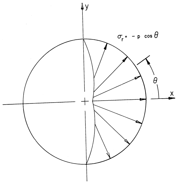
bjsfm.lekhnitskii.LoadedHole(load: float, diameter: float, thickness: float, a_inv: <sphinx.ext.autodoc.importer._MockObject object at 0x7f270bb34040>, theta: float = 0.0)¶ Class for defining a loaded hole in an infinite anisotropic homogeneous plate
A cosine bearing load distribution is assumed to apply to the inside of the hole.
Notes
Bearing distribution as shown below Ref. [4]
Parameters: - load (float) – bearing force
- diameter (float) – hole diameter
- thickness (float) – plate thickness
- a_inv (array_like) – 2D array (3, 3) inverse CLPT A-matrix
- theta (float, optional) – bearing angle counter clock-wise from positive x-axis (radians)
-
p¶ bearing force
Type: float
-
theta¶ bearing angle counter clock-wise from positive x-axis (radians)
Type: float
-
A¶ real part of equilibrium constant for first stress function
Type: float
-
A_bar¶ imaginary part of equilibrium constant for first stress function
Type: float
-
B¶ real part of equilibrium constant for second stress function
Type: float
-
B_bar¶ imaginary part of equilibrium constant for second stress function
Type: float
-
alpha() → <sphinx.ext.autodoc.importer._MockObject object at 0x7f270bb34040>¶ Fourier series coefficients modified for use in stress function equations
Notes
Exact solution:
\[\frac{P}{2\pi}\int_{-\pi/2}^{\pi/2} \cos^2 \theta \left( \cos m*\theta - i \sin m*\theta \right) \,d\theta\]\[= \frac{-2 P sin(\pi m/2)}{\pi m(m^2-4)}\]Modifications to the Fourier series coefficients are developed in Eq. 37.2 [2]
Returns: Return type: ndarray
-
beta() → <sphinx.ext.autodoc.importer._MockObject object at 0x7f270bb34040>¶ Fourier series coefficients modified for use in stress function equations
Notes
Exact solution:
\[\frac{-P}{2\pi}\int_{-\pi/2}^{\pi/2}\cos\theta\sin\theta\left(\cos m*\theta - i \sin m*\theta\right)\,d\theta\]\[= -\frac{i P sin(\pi m/2)}{\pi (m^2-4)}\]Modifications to the Fourier series coefficients are developed in Eq. 37.2 [2]
Returns: Return type: complex ndarray
-
equilibrium_constants() → tuple¶ Solve for constants of equilibrium
When the plate has loads applied that are not in equilibrium, the unbalanced loads are reacted at infinity. This function solves for the constant terms in the stress functions that account for these reactions.
Notes
This method implements Eq. 37.5 [2]. Complex terms have been expanded and resolved for A, A_bar, B and B_bar (setting Py equal to zero).
Returns: [A, A_bar, B, B_bar] – real and imaginary parts of constants A and B Return type: tuple
-
phi_1(z1: <sphinx.ext.autodoc.importer._MockObject object at 0x7f270bb34040>) → <sphinx.ext.autodoc.importer._MockObject object at 0x7f270bb34040>¶ Calculates the first stress function
Notes
This method implements [Eq. 37.3, Ref. 2]
\[C_m=\frac{\beta_m-\mu_2\alpha_m}{\mu_1-\mu_2}\]\[\Phi_1=A\ln{\xi_1}+\sum_{m=1}^{\infty}\frac{C_m}{\xi_1^m}\]Parameters: z1 (ndarray) – 1D complex array first mapping parameter Returns: 1D complex array Return type: ndarray
-
phi_1_prime(z1: <sphinx.ext.autodoc.importer._MockObject object at 0x7f270bb34040>) → <sphinx.ext.autodoc.importer._MockObject object at 0x7f270bb34040>¶ Calculates derivative of the first stress function
Notes
This method implements [Eq. 37.6, Ref. 2]
\[C_m=\frac{\beta_m-\mu_2\alpha_m}{\mu_1-\mu_2}\]\[\eta_1=\pm\sqrt{z_1^2-a^2-\mu_1^2b^2}\]\[\Phi_1'=-\frac{1}{\eta_1}(A-\sum_{m=1}^{\infty}\frac{m C_m}{\xi_1^m})\]Parameters: z1 (ndarray) – 1D complex array first mapping parameter Returns: 1D complex array Return type: ndarray
-
phi_2(z2: <sphinx.ext.autodoc.importer._MockObject object at 0x7f270bb34040>) → <sphinx.ext.autodoc.importer._MockObject object at 0x7f270bb34040>¶ Calculates the second stress function
Notes
This method implements [Eq. 37.3, Ref. 2]
\[C_m=\frac{\beta_m-\mu_1\alpha_m}{\mu_1-\mu_2}\]\[\Phi_2=B\ln{\xi_2}-\sum_{m=1}^{\infty}\frac{m C_m}{\xi_2^m}\]Parameters: z2 (ndarray) – 1D complex array second mapping parameter Returns: 1D complex array Return type: ndarray
-
phi_2_prime(z2: <sphinx.ext.autodoc.importer._MockObject object at 0x7f270bb34040>) → <sphinx.ext.autodoc.importer._MockObject object at 0x7f270bb34040>¶ Calculates derivative of the second stress function
Notes
This method implements [Eq. 37.6, Ref. 2]
\[C_m=\frac{\beta_m-\mu_1\alpha_m}{\mu_1-\mu_2}\]\[\eta_2=\pm\sqrt{z_2^2-a^2-\mu_2^2b^2}\]\[\Phi_2'=-\frac{1}{\eta_2}(B+\sum_{m=1}^{\infty}\frac{m C_m}{\xi_2^m})\]Parameters: z2 (ndarray) – 1D complex array second mapping parameter Returns: 1D complex array Return type: ndarray
-
stress(x: <sphinx.ext.autodoc.importer._MockObject object at 0x7f270bb34040>, y: <sphinx.ext.autodoc.importer._MockObject object at 0x7f270bb34040>) → <sphinx.ext.autodoc.importer._MockObject object at 0x7f270bb34040>¶ Calculates the stress at (x, y) points in the plate
Parameters: - x (array_like) – 1D array x locations in the cartesian coordinate system
- y (array_like) – 1D array y locations in the cartesian coordinate system
Returns: [[sx0, sy0, sxy0], [sx1, sy1, sxy1], … , [sxn, syn, sxyn]] (n, 3) in-plane stress components in the cartesian coordinate system
Return type: ndarray
-
class
bjsfm.lekhnitskii.UnloadedHole(loads: <sphinx.ext.autodoc.importer._MockObject object at 0x7f270bb34040>, diameter: float, thickness: float, a_inv: <sphinx.ext.autodoc.importer._MockObject object at 0x7f270bb34040>)¶ Class for defining an unloaded hole in an infinite anisotropic homogeneous plate
This class represents an infinite anisotropic plate with a unfilled circular hole loaded at infinity with forces in the x, y and xy (shear) directions.
Parameters: - loads (array_like) – 1D array [Nx, Ny, Nxy] force / unit length
- diameter (float) – hole diameter
- thickness (float) – laminate thickness
- a_inv (array_like) – 2D array (3, 3) inverse CLPT A-matrix
-
applied_stress¶ [\(\sigma_x^*, \sigma_y^*, \tau_{xy}^*\)] stresses applied at infinity
Type: (1, 3) ndarray
-
alpha() → complex¶ Calculates the alpha loading term for three components of applied stress at infinity
Three components of stress are [\(\sigma_{x}^*, \sigma_{y}^*, \tau_{xy}^*\)]
Notes
This method implements Eq. A.7 [1] which is a combination of Eq. 38.12 & Eq. 38.18 [2]
\[\alpha_1=\frac{r}{2}(\tau_{xy}^*i-\sigma_{y}^*)\]Returns: first fourier series term for applied stress at infinity Return type: complex
-
beta() → complex¶ Calculates the beta loading term for three components of applied stress at infinity
Three components of stress are [\(\sigma_x^*, \sigma_y^*, \tau_{xy}^*\)]
Notes
This method implements Eq. A.7 [1] which is a combination of Eq. 38.12 & Eq. 38.18 [2]
\[\beta_1=\frac{r}{2}(\tau_{xy}^*-\sigma_x^*i)\]Returns: first fourier series term for applied stresses at infinity Return type: complex
-
phi_1(z1: <sphinx.ext.autodoc.importer._MockObject object at 0x7f270bb34040>) → <sphinx.ext.autodoc.importer._MockObject object at 0x7f270bb34040>¶ Calculates the first stress function
Notes
This method implements Eq. A.6 [1]
\[C_1=\frac{\beta_1-\mu_2\alpha_1}{\mu_1-\mu_2}\]\[\Phi_1=\frac{C_1}{\xi_1}\]Parameters: z1 (ndarray) – 1D complex array first mapping parameter Returns: 1D complex array Return type: ndarray
-
phi_1_prime(z1: <sphinx.ext.autodoc.importer._MockObject object at 0x7f270bb34040>) → <sphinx.ext.autodoc.importer._MockObject object at 0x7f270bb34040>¶ Calculates derivative of the first stress function
Notes
This method implements Eq. A.8 [1]
\[C_1=\frac{\beta_1-\mu_2\alpha_1}{\mu_1-\mu_2}\]\[\eta_1=\frac{z_1\pm\sqrt{z_1^2-a^2-\mu_1^2b^2}}{a-i\mu_1b}\]\[\kappa_1=\frac{1}{a-i\mu_1b}\]\[\Phi_1'=-\frac{C_1}{\xi_1^2}(1+\frac{z_1}{\eta_1})\kappa_1\]Parameters: z1 (ndarray) – 1D complex array first mapping parameter Returns: 1D complex array Return type: ndarray
-
phi_2(z2: <sphinx.ext.autodoc.importer._MockObject object at 0x7f270bb34040>) → <sphinx.ext.autodoc.importer._MockObject object at 0x7f270bb34040>¶ Calculates the second stress function
Notes
This method implements Eq. A.6 [1]
\[C_2=-\frac{\beta_1-\mu_1\alpha_1}{\mu_1-\mu_2}\]\[\Phi_2=\frac{C_2}{\xi_2}\]Parameters: z2 (ndarray) – 1D complex array second mapping parameter Returns: 1D complex array Return type: ndarray
-
phi_2_prime(z2: <sphinx.ext.autodoc.importer._MockObject object at 0x7f270bb34040>) → <sphinx.ext.autodoc.importer._MockObject object at 0x7f270bb34040>¶ Calculates derivative of the second stress function
Notes
This method implements Eq. A.8 [1]
\[C_2=-\frac{\beta_1-\mu_1\alpha_1}{\mu_1-\mu_2}\]\[\eta_2=\frac{z_2\pm\sqrt{z_2^2-a^2-\mu_2^2b^2}}{a-i\mu_2b}\]\[\kappa_2=\frac{1}{a-i\mu_2b}\]\[\Phi_2'=-\frac{C_2}{\xi_2^2}(1+\frac{z_2}{\eta_2})\kappa_2\]Parameters: z2 (ndarray) – 1D complex array second mapping parameter Returns: 1D complex array Return type: ndarray
-
stress(x: <sphinx.ext.autodoc.importer._MockObject object at 0x7f270bb34040>, y: <sphinx.ext.autodoc.importer._MockObject object at 0x7f270bb34040>) → <sphinx.ext.autodoc.importer._MockObject object at 0x7f270bb34040>¶ Calculates the stress at (x, y) points in the plate
Parameters: - x (array_like) – 1D array x locations in the cartesian coordinate system
- y (array_like) – 1D array y locations in the cartesian coordinate system
Returns: [[sx0, sy0, sxy0], [sx1, sy1, sxy1], … , [sxn, syn, sxyn]] (n, 3) in-plane stress components in the cartesian coordinate system
Return type: ndarray
-
bjsfm.lekhnitskii.rotate_complex_parameters(mu1: complex, mu2: complex, angle: float = 0.0) → tuple¶ Rotates the complex parameters by given angle
The rotation angle is positive counter-clockwise from the positive x-axis in the cartesian xy-plane.
Notes
Implements Eq. 10.8 [2]
Parameters: - mu1 (complex) – first complex parameter
- mu2 (complex) – second complex parameter
- angle (float, default 0.) – angle measured counter-clockwise from positive x-axis (radians)
Returns: mu1p, mu2p – first and second transformed complex parameters
Return type: complex
-
bjsfm.lekhnitskii.rotate_material_matrix(a_inv: <sphinx.ext.autodoc.importer._MockObject object at 0x7f270bb34040>, angle: float = 0.0) → <sphinx.ext.autodoc.importer._MockObject object at 0x7f270bb34040>¶ Rotates the material compliance matrix by given angle
The rotation angle is positive counter-clockwise from the positive x-axis in the cartesian xy-plane.
Notes
This function implements Eq. 9.6 [1]
Parameters: - a_inv (ndarray) – 2D (3, 3) inverse CLPT A-matrix
- angle (float, default 0.) – angle measured counter-clockwise from positive x-axis (radians)
Returns: 2D (3, 3) rotated compliance matrix
Return type: ndarray
-
bjsfm.lekhnitskii.rotate_strain(strains: <sphinx.ext.autodoc.importer._MockObject object at 0x7f270bb34040>, angle: float = 0.0) → <sphinx.ext.autodoc.importer._MockObject object at 0x7f270bb34040>¶ Rotates 2D strain components by given angle
The rotation angle is positive counter-clockwise from the positive x-axis in the cartesian xy-plane.
Parameters: - strains (ndarray) – 2D nx3 array of [:math: epsilon_x, epsilon_y, epsilon_{xy}] in-plane strains
- angle (float, default 0.) – angle measured counter-clockwise from positive x-axis (radians)
Returns: 2D nx3 array of [:math: epsilon_x’, epsilon_y’, epsilon_{xy}’] rotated stresses
Return type: ndarray
-
bjsfm.lekhnitskii.rotate_stress(stresses: <sphinx.ext.autodoc.importer._MockObject object at 0x7f270bb34040>, angle: float = 0.0) → <sphinx.ext.autodoc.importer._MockObject object at 0x7f270bb34040>¶ Rotates 2D stress components by given angle
The rotation angle is positive counter-clockwise from the positive x-axis in the cartesian xy-plane.
Parameters: - stresses (ndarray) – 2D nx3 array of [:math: sigma_x, sigma_y, tau_{xy}] in-plane stresses
- angle (float, default 0.) – angle measured counter-clockwise from positive x-axis (radians)
Returns: 2D nx3 array of [:math: sigma_x’, sigma_y’, tau_{xy}’] rotated stresses
Return type: ndarray
Plotting Module
-
bjsfm.plotting.plot_stress(lk_1: Union[bjsfm.lekhnitskii.LoadedHole, bjsfm.lekhnitskii.UnloadedHole], lk_2: Union[bjsfm.lekhnitskii.LoadedHole, bjsfm.lekhnitskii.UnloadedHole] = None, comp: Union[x, y, xy] = 'x', rnum: int = 100, tnum: int = 100, axes: <sphinx.ext.autodoc.importer._MockObject object at 0x7f270bb7e400> = None, xbounds: tuple = None, ybounds: tuple = None, cmap: str = 'jet', cmin: float = None, cmax: float = None) → None¶ Plots stresses
Notes
- colormap options can be found at
- https://matplotlib.org/3.1.1/tutorials/colors/colormaps.html
Parameters: - lk_1 (bjsfm.lekhnitskii.UnloadedHole or bjsfm.lekhnitskii.LoadedHole) – LoadedHole or UnloadedHole instance
- lk_2 (bjsfm.lekhnitskii.UnloadedHole or bjsfm.lekhnitskii.LoadedHole, optional) – LoadedHole or UnloadedHole instance
- comp ({'x', 'y', 'xy'}, default 'x') – stress component
- rnum (int, default 100) – number of points to plot along radius
- tnum (int, default 100) – number of points to plot along circumference
- axes (matplotlib.axes, optional) – a custom axes to plot on
- xbounds (tuple of float, optional) – (x0, x1) x-axis bounds, default=6*radius
- ybounds (tuple of float, optional) – (y0, y1) y-axis bounds default=6*radius
- cmap (str, optional) – name of any colormap name from matplotlib.pyplot
- cmin (float, optional) – minimum value for colormap
- cmax (float, optional) – maximum value for colormap